Cookbook

Below we offer some complete examples, with sample input data, which demonstrate some of the functionality and expected outputs.

Analysis of RX Eridanus

RX Eridanus is a variable star with known variability so it makes for an ideal demonstration of AstroSource. The data we present shows variability but also has noise, so don’t be alarmed by that.

The sample dataset is a time-series of photometry data of the variable star RX Eridanus. The data was taken by Michael Fitzgerald and Tim Jones on Las Cumbres Observatory’s 0.4-meter optical telescopes in 2018-2019. The photometry has been extracted via a source extraction algorithm and for each image is saved into a corresponding CSV format file with the extension .psx.

Sample data

Download data set from FigShare.

There are no FITS or other image files in this zip archive. All of the data are photometry tables saved in CSV format.

Once you have downloaded this data, unzip it.

Using Command Line Interface

To use the command line interface (CLI) to perform the

$ astrosource \
--ra 72.43451 \
--dec -15.74109 \
--format psx \
--indir <PATH TO DATA> \
--full

Because we have a text file in CSV format with the extracted photometry, and not FITS file with the photmetry in a FITS Table, we need to explicitly tell astrosource which file extension to look for. astrosource will assume that every file in indir with the extension provided is one of our astrometry data files.

--full

This is shorthand for running astrosource with the following options:

--stars \
--comparison \
--calc \
--phot \
--plot

Outputs

These are the output lightcurves, found in outputplots/ for this dataset.

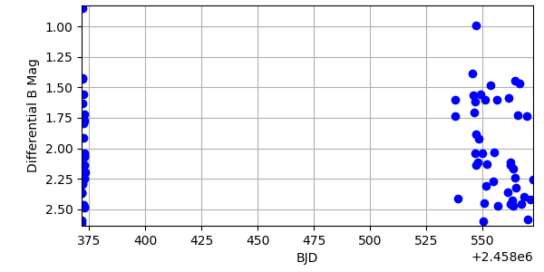
Differential Magnitude lightcurve

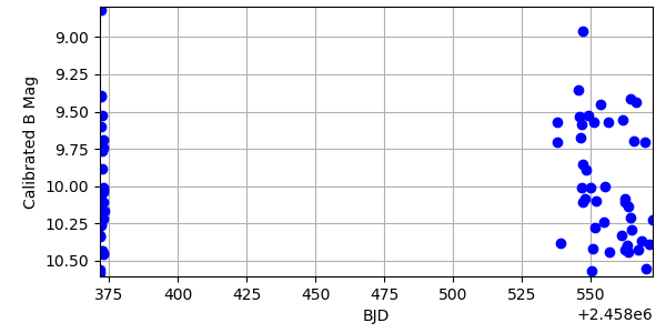
astrosource automatically will attempt to perform calibrated lightcurve calculations. It does this by making an API call to online astronomical catalogues via the Python package astroquery. If you are offline when you run astrosource you will not get a calibrated lightcurve.

The main issue with the dataset can be seen easily in this figures. The lightcurve has a large gap because the data were taken at 2 distinct epochs.

Period Folding

For a periodic timeseries, like variable stars or eclipsing binaries, astrosource has a period fitting feature. Using CLI you will have to run the full pipeline again with following inputs:

--period \
--periodlower 0.2 \
--periodupper 1.0

Set reasonable guesses for the boundaries of your source. Having the –periodlower and –periodupper close to each other increases the resolution of the finding algorithm, which uses 10,000 steps between these bounds.

This makes our full astrosource call the following:

$ astrosource \
--ra 72.43451 \
--dec -15.74109 \
--format psx \
--indir <PATH TO DATA> \
--period \
--periodlower 0.2 \
--perdioupper 1.0
--full

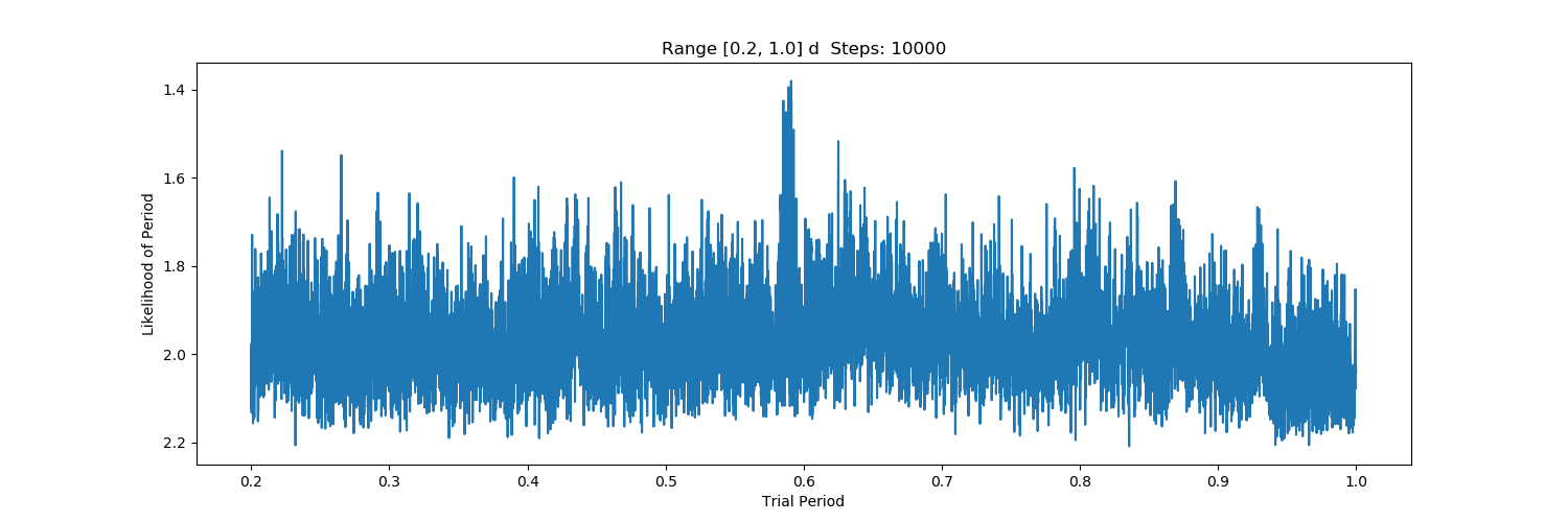
The outputs can be found in periods/. astrosource calculates the period via Phase Dispersion Minimization (PDM).

First the maximum likelihood plot for all the possible periods in the range provided, where you can see a peak at ~0.6 days.

Then the phase folded data, using the obtained period. We provide 2 identical traces of the data making it easier to see trends.

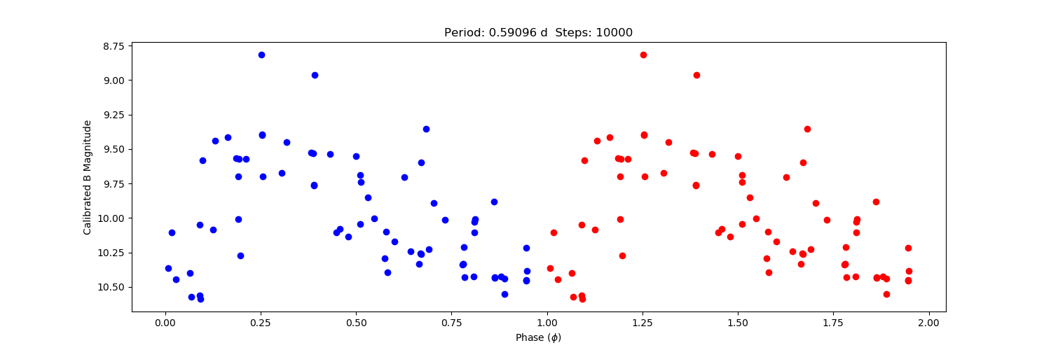
You can see that the estimated period is 0.59096 days. The published value is 0.58725159 days in an ApJ Letter.